TP Theorical Chemistry: 2S-3e bonds in proteins


Date: December 2018

E. Dumont


This practical aims at using and applying the methods that were described during the lectures. We will use the Gaussian package (online help). Calculations will be launched on the machines of CBP. Visualization of geometries and inspection of molecular orbital will be done with molden, avogadro or Gabedit depending on your liking.
We will be interesting into the one-electron attachment onto disulfides. This is an ubiquitous "reaction" for proteins, notably of the thioredoxin superfamily which act as a molecular rheostat in cells. The cartoon representation is given below:

some_text

Here is a summary of what we will survey:


We first explore the level of theory suited to reproduce the electron affinity and optical properties of the electron attachment on disulfide. During a second practical, we will investigate the same "reaction" within protein relying on a QM/MM approach.


1. Specific requirements for a correct basis set ?
  1. Build up the dimethyldisulfide molecule with your favorite builder.
  2. Optimize its geometry at the HF/6-31G* level of theory for the neutral (N) and radical anionic (RA) states. Which vertical and adiabatic electron affinities do you infer at this level of theory ? What is the main geometrical change upon electron attachment. Discuss the geometrical evolution and compare to the X-ray structure of an irradiated protein described in this paper: Weik and coworkers, PNAS, 2000, link. (To submit the job g09 dmeds.com dmeds.log should work and open the result file H2.log. The input can look like:
    # nosymm hf/6-31G* gen opt=tight scf=tight
    
    DMeDS
    
    0 1 
     C      .000000      .000000      .000000
     H      .000000      .000000     1.008000
     H     1.026719      .000000     -.363000
     H     -.513360     -.889165     -.363000
     S    -1.074802      .000000    -1.330000
     S    -2.988705      .000000     -.653333
     C    -4.063507      .000000    -1.983333
     H    -5.090226      .000000    -1.620333
     H    -3.892387      .889165    -2.588333
     H    -3.892387     -.889165    -2.588333
    
    -- the infamous blank line -- 
    
    
  3. The experimental adiabatic electron affinity (AEA) is of 0.10 eV for dimethyldisulfide: what is missing in our description ?
  4. Redo the calculation with the 6-31+G* basis set. What is the difference with the former 6-31G* basis set ?
  5. To estimate the convergence, one can compare with the "golden standard" triple-zeta Dunning's basis set aug-cc-pVTZ. The outputs are given because the calculations are becoming larger (N-opt-hf-tz.log and RA-opt-hf-tz.log).
  6. To avoid a prohibitve use of this reference basis set, Schaefer and coworkers have proposed a intermediate-size yet equal-performance basis set, DZP++. It does not belong to the standard basis set provided by Gaussian. Relaunch the calculations for the neutral and radical anionic states. Hos the AEA situates at this level of theory ?
  7. The experimental adiabatic electron affinity (AEA) is of 0.10 eV for dimethyldisulfide: what is missing in our description ?
  8. Redo the calculations with the MP2 method, i.e. the second-order Moller-Plesset perturbation theory approach. Do geometries change ? does the AEA estimation changes ? (Be careful... The "SCF Done" line provides the Hartree-Fock energy, you need to look for EMP2 = , EUMP2 = ).
  9. A quoi correspond la valeur S**2 ?

In passing, feel free to identify the various steps of the Gaussian calculation with the reference to the various links, whose specification is given on Gaussian website online, (e.g. /softs/gaussian/g03a02/g09/l1.exe, which you can search Link in the output file).

 
- (Enter /softs/gaussian/g03a02/g09/l101.exe) Reads title and molecule specification
- (Enter /softs/gaussian/g03a02/g09/l202.exe) Reorients coordinates, calculates symmetry,
and checks variables
- (Enter /softs/gaussian/g03a02/g09/l301.exe) Generates basis set information
- (Enter /softs/gaussian/g03a02/g09/l302.exe) Calculates overlap, kinetic, and potential
integrals
- (Enter /softs/gaussian/g03a02/g09/l303.exe) Calculates multipole integrals
- (Enter /softs/gaussian/g03a02/g09/l401.exe) Forms the initial MO guess
- (Enter /softs/gaussian/g03a02/g09/l502.exe) Iteratively solves the SCF equations
- (Enter /softs/gaussian/g03a02/g09/l601.exe) Population and related analyses
- (Enter /softs/gaussian/g03a02/g09/l9999.exe) Finalizes calculation and output

As an aparte, one can also notes that in some QM software, basis sets are not localized but described as plane waves, which avoids the awful acronyms and the lack of systematic behavior. On the other hand, here one could choose to treat the sulfurs with diffuse functions to save a bit the computation time.


2. Three-electron two-center bonding: a test case for DFT.


DFT comes with a rather accurate treatment of electron correlation which can trigger some ameliorations to our QM description of 2S-3e. On the other hand, density functionals are fitted on even-number systems and radicals often requires a more careful description. Also radical systems tend to be more multi-reference. For this system, one can compute a T1 diagnostic to ensure the mono-referential description makes sense.
  1. Optimize the two species into play and estimate the electron affinity. Each of you can use functional and you will share the results: BLYP, B3LYP, LC-BLYP. The basis set 6-31+G** will be used (DFT is less sensitive to basis set than HF and post-HF methods). In gas phase, the experimental value for the adiabatic electron affinity is estimated to 0.1 eV. Discuss the numerical agreement. Which functional singles out ?
  2. Where goes the additional electron ? Provide an orbital explanation. Is there an analog of the Koopmans theorem to predict AEA here ?
  3. Discuss the geometry evolution and compare to the X-ray structure of an irradiated protein described in this paper: Weik and coworkers, PNAS, 2000, link.
  4. Add an implicit solvent (keyword: scrf=pcm, water is the default). Is this the trend you were expecting ?


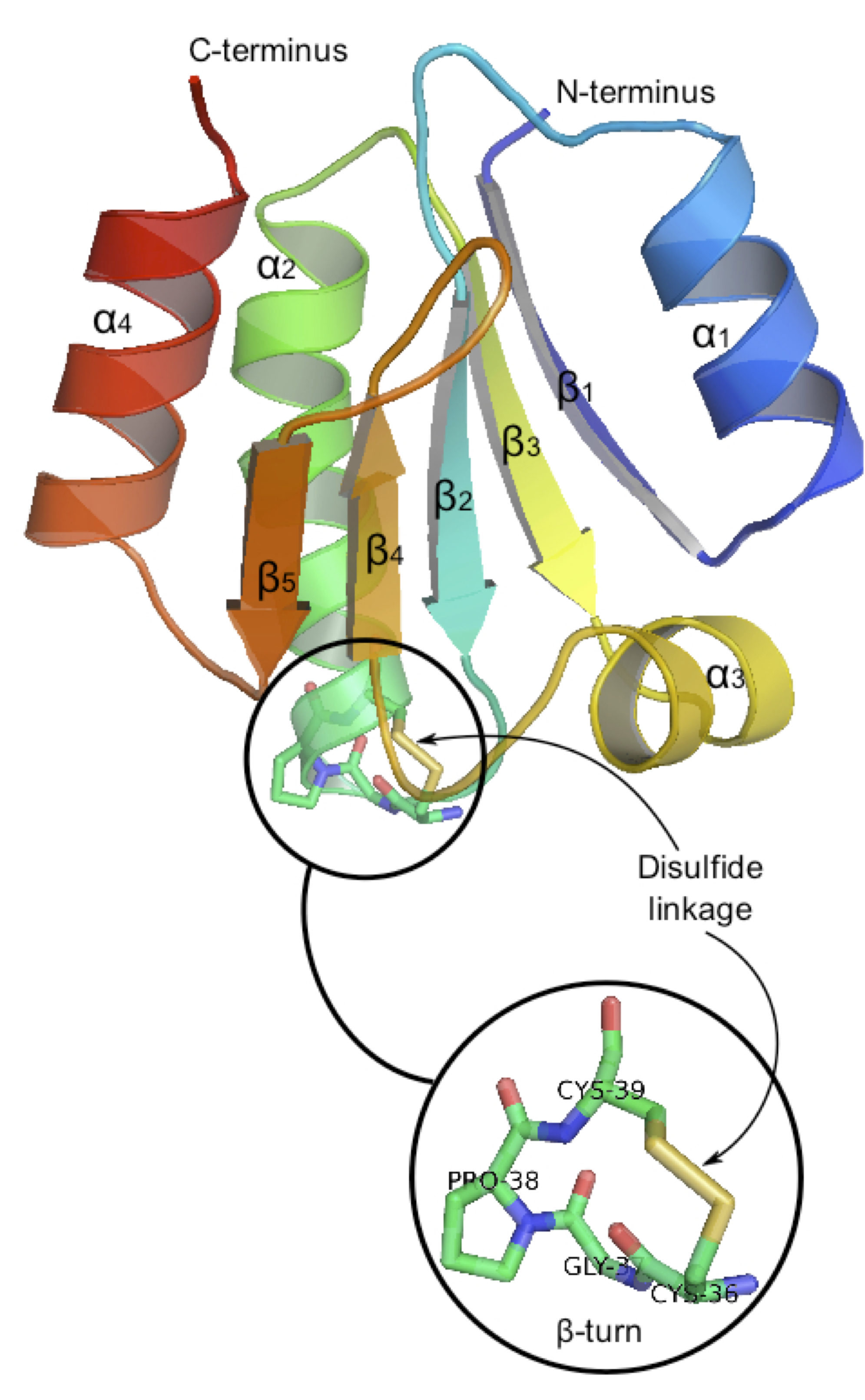
3. Solvation


Within proteins, disulfide bridges are often strongly solvent-exposed (to water). We are going to test the several implicit models (before QM/MM...).
  1. What quantity can be measured ? How would you reproduce it ? (The adiabatic electron affinity may not be the most relevant quantity...)
  2. Launch the geometry optimizations this time using an implicit solvation model. Which ones are available within Gaussian ? (You might be using using G09 instead of G16 with some new features).
  3. How evolves the AEA ? Is it expected ? (Absolute energies differ a lot... that's normal).

Each group can try: scrf=pcm, SCRF=(Dipole,solvent=water,A0=3.71) (the Onsager model), SCRF=smd (Truhlar's model), SCRF=(sas) to compare several approaches.


4. Optical properties


The identification of 2S-3e in biological molecules relies on a characteristic UV-Vis signature σ -> σ* at 410nm in water.
  1. Perform a TDDFT calculation on the optimized geometry at the MP2/6-31+G* level of theory to situate the transition HOMO-LUMO of the radical anion and of the neutral moities. Indication: each student could take one or two different functionals.
  2. Verify the transition type by studying the orbitals.

Results Results HF+DFT (notebook by the student)


List of coefficients for the DZP++ basis set

H     0
S   3   1.00
     19.2406000              0.0328280
      2.8992000              0.2312080
      0.6534000              0.8172380
S   1   1.00
      0.1776000              1.0000000
P   1   1.00
      1.0000000              1.0000000
P   1   1.00
      0.7500000              1.0000000
S   1   1.00
      0.0441500              1.0000000
****
C     0
S   6   1.00
   4232.6100000              0.0020290
    634.8820000              0.0155350
    146.0970000              0.0754110
     42.4974000              0.2571210
     14.1892000              0.5965550
      1.9666000              0.2425170
S   1   1.00
      5.1477000              1.0000000
S   1   1.00
      0.4962000              1.0000000
S   1   1.00
      0.1533000              1.0000000
P   4   1.00
     18.1557000              0.0185340
      3.9864000              0.1154420
      1.1429000              0.3862060
      0.3594000              0.6400890
P   1   1.00
      0.1146000              1.0000000
D   1   1.00
      0.7500000              1.0000000
S   1   1.00
      0.0430200              1.0000000
P   1   1.00
      0.0362900              1.0000000 
**** 
S     0 
S   5   1.00
  35710.0000000              0.0025650 
   5397.0000000              0.0194050
   1250.0000000              0.0955950 
    359.9000000              0.3457930
    119.2000000              0.6357940 
S   3   1.00
    119.2000000              0.1300960
     43.9800000              0.6513010
     17.6300000              0.2719550 
S   1   1.00
      5.4200000              1.0000000 
S   1   1.00
      2.0740000              1.0000000
S   1   1.00
      0.4246000              1.0000000
S   1   1.00
      0.1519000              1.0000000
P   4   1.00
    212.9000000              0.0140910 
     49.6000000              0.0966850
     15.5200000              0.3238740
      5.4760000              0.6917560
P   2   1.00
      5.4760000             -0.6267370 
      2.0440000              1.3770510 
P   1   1.00
      0.5218000              1.0000000 
P   1   1.00
      0.1506000              1.0000000
D   1   1.00
      0.7000000              1.0000000
S   1   1.00
      0.0426700              1.0000000
P   1   1.00
      0.0409600              1.0000000
****


Last update : Dec. 2018