Deformation estimations on a moving racing car recording
Copyright (C) 2017 Adrien MEYNARD
This program is free software; you can redistribute it and/or modify it under the terms of the GNU General Public License as published by the Free Software Foundation; either version 3 of the License, or (at your option) any later version.
This program is distributed in the hope that it will be useful, but WITHOUT ANY WARRANTY; without even the implied warranty of MERCHANTABILITY or FITNESS FOR A PARTICULAR PURPOSE. See the GNU General Public License for more details.
You should have received a copy of the GNU General Public License along with this program. If not, see http://www.gnu.org/licenses/.
Author: Adrien MEYNARD Email: adrien.meynard@univ-amu.fr Created: 2017-12-19
Contents
Load signal
clear all; close all; clc;

warning off;
addpath('cwt');
addpath('deform_estimation');

load('signals/doppler_f1');
T = length(y);
Joint estimation
Dt = 100; % temporal subsampling for the deformation estimation
dgamma0 = ones(1,T); % gamma'(t) initialization
a0 = ones(1,T); % a(t) initialization

wav_typ = 0; % wavelet type (cf. cwt.m)
wav_paramWP = 20; % corresponding parameter for warping estimation
wav_param = 500; % corresponding parameter for spectrum and AM estimations

NbScales = 125;
scalesAM = 2.^(linspace(1,6,NbScales));
subrate = 3; % subsampling step for the scales to ensure the covariance invertibility
scalesWP = scalesAM(1:subrate:end);

stopWP = 2e-2; % minimal gap between two steps in the gradient
itWP = 6; % number of gradient iterations

r = 1e-5; % regularization parameter

Nf = 2500; % number of frequencies for spectrum estimation
NbScalesS = 110;
scalesS = 2.^(linspace(-1,7,NbScalesS)); % for spectrum estimation

Nit = 10; % maximal number of iterations in the joint estimation
stop_crit = 5e-3; % relative update threshold

paramWAV = {wav_typ,wav_param,wav_paramWP};
paramAM = {'AM',scalesAM,r}; % AM (model without noise)
paramWP = {scalesWP,itWP,stopWP};
paramS = {scalesS,Nf};

% AM + WP estimation
fprintf('\nJoint AM and Time Warping estimation: \n\n')
tic;
[aML, dgammaML, Sx, evol_crit] = estim_altern(y,Dt,dgamma0,a0,paramWAV,paramWP,paramAM,paramS,stop_crit,Nit);
toc;

% WP estimation only
fprintf('\nTime Warping estimation only (model without AM): \n\n')
paramAM2 = {'no AM'}; % model with time warping only
tic;
[aML2, dgammaML2, Sx2, evol_crit2] = estim_altern(y,Dt,dgamma0,a0,paramWAV,paramWP,paramAM2,paramS,stop_crit,Nit);
toc;
Joint AM and Time Warping estimation:

 Iteration 1
 Relative update WP: Inf %
 Relative update AM: 44.80 %

 Iteration 2
 Relative update WP: 86.91 %
 Relative update AM: 38.02 %

 Iteration 3
 Relative update WP: 280.35 %
 Relative update AM: 8.91 %

 Iteration 4
 Relative update WP: 166.05 %
 Relative update AM: 6.56 %

 Iteration 5
 Relative update WP: 4.92 %
 Relative update AM: 31.46 %

 Iteration 6
 Relative update WP: 2.84 %
 Relative update AM: 0.61 %

 Iteration 7
 Relative update WP: 0.02 %
 Relative update AM: 0.00 %

Elapsed time is 366.447932 seconds.

Time Warping estimation only (model without AM):

 Iteration 1
 Relative update WP: Inf %

 Iteration 2
 Relative update WP: 287.05 %

 Iteration 3
 Relative update WP: 256.44 %

 Iteration 4
 Relative update WP: 2.36 %

 Iteration 5
 Relative update WP: 0.01 %

Elapsed time is 207.332860 seconds.
Wavelet transforms
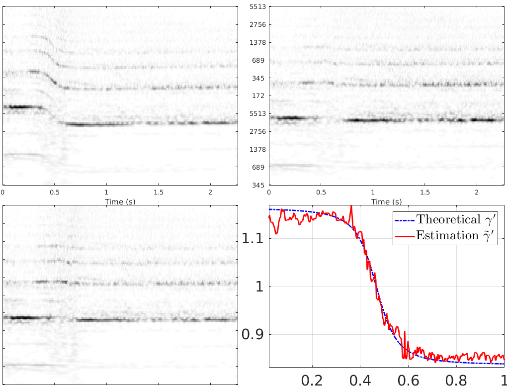
addpath('analysis');

z = statAMWP(y,aML,dgammaML); % AM + WP estimations => stationarization
z2 = statAMWP(y,aML2,dgammaML2); % WP estimation only => stationarization

Wy = cwt(y,scalesAM,0,wav_param);
Wz = cwt(z,scalesAM,0,wav_param);
Wz2 = cwt(z2,scalesAM,0,wav_param);

t = linspace(0,(T-1)/Fs,T);

figure;
subplot('Position', [0.005 0.52, 0.465, 0.465]);
imagesc(t,log2(scalesAM),abs(Wy));
xlabel('Time (s)')
set(gca,'yticklabel',[])

p = subplot('Position', [0.53 0.52, 0.465, 0.465]);
imagesc(t,log2(scalesAM),abs(Wz));
xi0 = Fs/4;
xlabel('Time (s)')
sobs = cellfun(@str2num,get(p,'yticklabel'));
fobs = round(xi0./2.^sobs);
set(gca,'yticklabel',fobs);
colormap(flipud(gray));

subplot('Position', [0.005 0.005, 0.465, 0.465]);
imagesc(t,log2(scalesAM),abs(Wz2));
set(gca,'yticklabel',[])
Doppler effect
c = 330;
v = 54;
d = 5;
L = 25.2;
dgammaTH = 1 + v.*(L-v.*t)./sqrt(d^2*(c^2-v.^2) + c^2*(L-v.*t).^2); % theoretical gamma'

dgammaMLn = 1.02*dgammaML*mean(dgammaTH)/mean(dgammaML); % /!\ normalization (gamma' is estimated up to a multiplicative factor)
p = subplot('Position', [0.53 0.05, 0.465, 0.42]);
plot(t,dgammaTH,'b-.',t,dgammaMLn,'r', 'linewidth',2); grid on; axis tight;
V = axis; axis([0.02 1 V(3) V(4)]);
legend({'Theoretical $\gamma''$','Estimation $\tilde\gamma''$'},'interpreter','latex')
set(gca, 'FontSize', 22);