Summer School EMIE – Part 1
Proton transfer and Microsolvation
Date: June 2023
C. Michel
Our aim is to investigate how a proton transfer can be tuned by the presence of water. We will use the software Gaussian (online manual). The preparation of input files and the visualisation of results will be done using Avogadro.
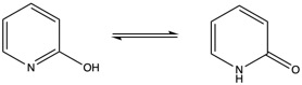
We will study the tautomerization reaction of 2-hydroxypyridine / 2-pyridone.
Our calculations will be performed at the PM6 level for the sake of efficiency. Comparison with experiments and other levels of calculations can be made by comparison with the reference article J. L. Sonnenberg et al. J. Chem. Theory Comput. 2009, 5, 4, 949-961 . The sequence is split in three steps and is expected to take 1h30.
1. Tautomerization in vacuum
We start by studying the reactant and product.
- Build the 2-pyridone (PY) and the 2-hydroxypyridine (HY) using Avogadro.
- Optimize those structures at the PM6 level using Gaussian and compute frequencies to get Gibbs free energies.
Here is a typical input file structure:#n PM6 Opt Freq [blanck line] [Title] Optimization of PY [blanck line] [Multiplicity,Charge] 0,1 [xyz formated coordinates] [blank line]
- Check the absence of an imaginary frequency using Avogadro or reading the .log file (NImag=).
- Determine the reaction energy. The Gibbs energy is reported in the - Thermochemistry - paragraph of the .log file as the Sum of electronic and thermal Free Energies= in Hartree/particle.
We move to the transition state search. We will first perform a scan along a well-chosen coordinate and consider that the structure at the highest energy is a good approximation of the TS structure, close enough to switch to a eigen-follow method to optimize the TS.
- Measure the N-H and O-H distance in both molecules and identify the labels of O, N, and the H to be transferred.
- Choose a starting structure and the variable to be used in the scan (typically O…H or N…H distance).
- Prepare the corresponding input file. You can follow this exemple that corresponds to stirring the N1-H8 distance in PY using 2 steps of 0.15 Å. Adapt the number of steps and the step size!
#n PM6 Opt=ModRedundant

H transfer py to HY

0,1
N  -1.135204 0.239458 0.000000
C  0.000000 1.069179 0.000000
C  1.244256 0.320141 0.000000
C  1.264957 -1.051903 0.000000
C  0.056462 -1.809209 0.000000
C  -1.129901 -1.126884 0.000000
O  -0.123527 2.292845 0.000000
H  -2.017014 0.740588 0.000000
H  2.157927 0.905065 0.000000
H  2.220524 -1.570494 0.000000
H  0.059757 -2.891970 0.000000
H -2.101193 -1.610110 0.000000

1 8 S 2 0.15
- You can plot the energy in function of the coordinate using this script which takes only the .log file as an argument and produces a image if the profile as a output, a table of the energies and the coordinates of the optimized structure at each step. If needed, you can refine the scan by adding more points close to the maximum: start from a structure close to this maximum that is provided by the script, and relauch a scan with smaller steps. If needed, change reaction coordinate, switching from N..H to O..H.
- Select the structure the closest to the maximum and optimize the transition state using the TS option in opt. The calcfc option allows to compute the hessian prior starting the optimization. The noeigentest allows to perform the optimisation even if more than one imaginary frequency is found in the starting hessian. You can try with and without those keywords.
#n PM6 Opt=(TS,calcfc,noeigentest) freq
- Check that the structure has been optimized and shows one and only one imaginary frequency. Visualize the corresponding mode of vibration.
Does it correspond to the reaction coordinate? - Determine the Gibbs free energy of activation of the tautomerization.
2. Using a continuum model
This tautomerization is known to be strongly facilitated by the presence of water. Repeat the previous calculation adding a continuum model for the water solvent adding the keyword SCRF=(Solvent=water). Compare the reaction energies and activation energies with the ones obtained in vacuum and conclude.
3. Microsolvation approach
We move now to a micro-solvation approach by adding water molecules. We start with one water molecule that can be H-bonded to O and/or to N:
- Determine the best structure with a water molecule H-bonded to PY in vacuum at the PM6 level of theory. Measure the NH…Ow and the Hw…O distances.
- Determine the best structure with a water molecule H-bonded to HY in vacuum at the PM6 level of theory. Measure the N…Hw and the OH…Ow distances.
- How is the reaction energy modified by the inclusion of a H-bonded water molecule?
- Determine the best transition state structure for the tautomerization.
- How is the reaction barrier modified by the inclusion of a H-bonded water molecule?
To ensure that most of the effect is indeed obtained using one water molecule, we need to investigate what happens with more water molecules and upon inclusion of a continuum model.
- Repeat with two water molecules.
- Repeat with three water molecules.
- Repeat including the PCM.
- Conclude.
Bonuses
- Let’s consider now methanol as a solvent. Is the H-transfer also assisted by this solvent?
- Can ammonia also catalyze this tautomerization ? See for instance J. Phys. Chem. A 2013, 117, 7523–7534.
- Can you propose an aromatic susbtitution that would favor the HY form?
- To move to a fully-explicit description of the water solvent, we could solvate the molecule in a box of liquid water and use ab initio metadynamics. Which collective variables would you suggest to use? Why?
- The PY/HYD can easily dimerize. How could you assess the impact of the solvent on this dimerization?
- In this dimer, the proton transfer is not observed in the ground state but can be observed in the exctited state. If interested, see Chemical Physics Letters
2019, 730, 634-637.
Some optimized structures in .xyz format
12
TS in vacuum
 N   -1.14643    0.15373   -0.00000
 C   -0.00000    0.98749   -0.00000
 C    1.29669    0.45162    0.00000
 C    1.39237   -0.93644    0.00000
 C    0.24893   -1.76106    0.00000
 C   -1.03284   -1.19466    0.00000
 O   -0.57315    2.14740   -0.00000
 H   -1.78463    1.40726   -0.00000
 H    2.16418    1.10316    0.00000
 H    2.38019   -1.40446    0.00000
 H    0.36258   -2.84078    0.00000
 H   -1.94292   -1.80223   -0.00000
15
TS with one water molecule
 C   -0.23694    0.68650   -0.01880
 C    1.03891    1.32241    0.01873
 C    2.16848    0.53222    0.03157
 C    2.05929   -0.87898    0.01037
 C    0.79986   -1.46218   -0.02365
 N   -0.34095   -0.70633   -0.03219
 H    3.16022    0.98842    0.05751
 H    1.07590    2.40881    0.03077
 H    2.95459   -1.49235    0.01835
 H    0.66295   -2.54918   -0.04390
 O   -1.35507    1.33415   -0.03129
 H   -2.38055    0.54579   -0.12789
 H   -3.05045   -0.70584    0.88617
 O   -2.80644   -0.62790   -0.04509
 H   -1.72159   -1.10113   -0.09384
18
TS with two water molecules
 N   -0.09023    0.60184   -0.00385
 C   -0.30033   -0.77024   -0.02935
 C   -1.62996   -1.30705   -0.02201
 C   -2.70025   -0.44488    0.00960
 C   -2.48379    0.95567    0.03613
 C   -1.18535    1.43502    0.03158
 O    0.71270   -1.56826   -0.05310
 H    1.87034   -1.09008   -0.13952
 H   -1.74049   -2.38907   -0.04273
 H   -3.72283   -0.82688    0.01480
 H   -3.32960    1.63549    0.06187
 H   -0.96477    2.50888    0.05793
 O    3.05526   -0.73380   -0.01221
 H    3.26549   -1.02110    0.88362
 H    2.92822    0.42801    0.06722
 O    2.29536    1.58299    0.03719
 H    1.20178    1.18505    0.05272
 H    2.41486    1.89834   -0.85958
21
TS with three water molecules
 N   -0.49753   -0.53204    0.22683
 C   -0.80998    0.80611    0.06022
 C   -2.15069    1.22941   -0.19997
 C   -3.14207    0.27662   -0.28479
 C   -2.82699   -1.09210   -0.11502
 C   -1.51154   -1.45406    0.13540
 O    0.13778    1.69352    0.14400
 H    1.24819    1.27276    0.36647
 H   -2.33953    2.29295   -0.32309
 H   -4.17521    0.56753   -0.48290
 H   -3.60760   -1.84319   -0.18188
 H   -1.21527   -2.50121    0.27370
 O    1.91836   -1.43378    0.66260
 H    0.87023   -1.03157    0.49043
 H    2.29488   -0.76661    1.28205
 O    3.05685   -0.42795   -1.26000
 H    2.46637   -1.13444   -0.45393
 H    3.98072   -0.65299   -1.13009
 O    2.49154    0.98336    0.55798
 H    2.89246    1.82425    0.73575
 H    2.87884    0.57973   -0.57588
Last update : June 2023