1. woody: model logflux

knitr::opts_chunk$set(warning=FALSE,message=FALSE)
library(woody)
library(tidyverse)
library(DiagrammeR)

Global process

For one site

Global process

For several sites

Here, we want to carry out this process for two sites, so that we use and enrich a nested table from step to step in the following manner:

We detail each step of this process afterwards.

Prepare data

tib_sites: info about wood and discharge data path, and hydrological stations

Prepare data describing the two stations:

tib_sites=tibble::tibble(site=c("Ain","Allier"),
                         q1.5=c(840,460),
                         station=c("V294201001 ","K340081001")) %>% 
  mutate(wpath=paste0("../data-raw/Wdata_",site),
         qpath=paste0("../data-raw/qtvar/q",site,".csv"))
tib_sites

## # A tibble: 2 × 5
##   site    q1.5 station       wpath                    qpath                     
##   <chr>  <dbl> <chr>         <chr>                    <chr>                     
## 1 Ain      840 "V294201001 " ../data-raw/Wdata_Ain    ../data-raw/qtvar/qAin.csv
## 2 Allier   460 "K340081001"  ../data-raw/Wdata_Allier ../data-raw/qtvar/qAllier…

`Wdata` : wood occurrence data

First step: import wood data , indicating path to files and site name:

We will obtain as a result tib_W= tib_sites completed with Wdata.

result_file="../data-raw/results/tib_W.RDS"
if(!file.exists(result_file)){
  tib_W=tib_sites %>% 
    group_by(vars=site,q1.5,station,wpath) %>% 
    mutate(Wdata=purrr::map2(.x=wpath,.y=site,
                             ~import_Wdata(path=.x,site=.y,
                                           min_length=1,
                                           sample_length=TRUE
                                           ))) %>% 
    mutate(Wdata=purrr::map(.x=Wdata,
                            ~mutate(.x,site=factor(site,levels=tib_sites$site))))
  saveRDS(tib_W,result_file)
}
tib_W=readRDS(result_file)

tib_W looks like this:

site	q1.5	station	wpath	qpath	vars	Wdata
Ain	840	V294201001	../data-raw/Wdata_Ain	../data-raw/qtvar/qAin.csv	Ain	10403 rows x 6 cols
Allier	460	K340081001	../data-raw/Wdata_Allier	../data-raw/qtvar/qAllier.csv	Allier	13806 rows x 6 cols

and inside tib_W, the first lines of Wdata (for both sites) look like this (here for the Ain site):

site	event	sitevent	Time	Length	Date
Ain	event_1	Ain_event_1	2007-11-22 14:20:56	1.51	2007-11-22
Ain	event_1	Ain_event_1	2007-11-22 14:58:13	1.53	2007-11-22
Ain	event_1	Ain_event_1	2007-11-22 14:58:49	4.13	2007-11-22
Ain	event_1	Ain_event_1	2007-11-22 15:09:53	5.29	2007-11-22
Ain	event_1	Ain_event_1	2007-11-22 16:20:35	1.32	2007-11-22
Ain	event_1	Ain_event_1	2007-11-23 06:56:44	3.79	2007-11-23

`Qdata`: collect hydrological data & calculate all variables

Collect qtvar data from banquehydro, for the period covered by Wdata, and back in time so as to be able to calculate \(T_Q\):

result_file="../data-raw/results/tib_WQ.RDS"
if(!file.exists(result_file)){
  tib_WQ=tib_W %>% 
    mutate(Qdata=purrr::map(.x=qpath,.y=site,
                            ~import_Qdata(path=.x, site=.y))) 
  saveRDS(tib_WQ,result_file)
}
tib_WQ=readRDS(result_file)

tib_WQ looks like this:

site	q1.5	station	wpath	qpath	vars	Wdata	Qdata
Ain	840	V294201001	../data-raw/Wdata_Ain	../data-raw/qtvar/qAin.csv	Ain	10403 rows x 6 cols	86528 rows x 4 cols
Allier	460	K340081001	../data-raw/Wdata_Allier	../data-raw/qtvar/qAllier.csv	Allier	13806 rows x 6 cols	82110 rows x 4 cols

and inside tib_WQ, the first lines of Qdata (for both sites) look like this:

## # A tibble: 6 × 4
##   station  Time                    Q site 
##   <chr>    <dttm>              <dbl> <chr>
## 1 V2942010 2001-01-01 00:00:00 113   Ain  
## 2 V2942010 2001-01-01 03:00:00 115   Ain  
## 3 V2942010 2001-01-01 04:48:00 112   Ain  
## 4 V2942010 2001-01-01 05:20:00 107   Ain  
## 5 V2942010 2001-01-01 06:06:00  99.8 Ain  
## 6 V2942010 2001-01-01 07:18:00  92   Ain

`Qdata` completed with calculation of \(T_Q\) and \(S\)

result_file="../data-raw/results/tib_WQc.RDS"
if(!file.exists(result_file)){
  tib_WQc=tib_WQ %>% 
    mutate(Qdata=purrr::map2(.x=Qdata,.y=q1.5,
                             ~complete_Qdata(qtvar=.x, qnorm=.y)))
  saveRDS(tib_WQc,result_file)
}
tib_WQc=readRDS(result_file)

tib_WQc looks like tib_WQ, except now Qdata inside has been completed with new variables:

head(tib_WQc$Qdata[[1]])

## # A tibble: 6 × 7
##   site  station  Time                    Q   T_Q          S  rT_Q
##   <chr> <chr>    <dttm>              <dbl> <dbl>      <dbl> <dbl>
## 1 Ain   V2942010 2001-01-01 00:00:00 0.135 0     NA         0    
## 2 Ain   V2942010 2001-01-01 03:00:00 0.137 0.125  0.0000661 0.354
## 3 Ain   V2942010 2001-01-01 04:48:00 0.133 0     -0.000165  0    
## 4 Ain   V2942010 2001-01-01 05:20:00 0.127 0     -0.000930  0    
## 5 Ain   V2942010 2001-01-01 06:06:00 0.119 0     -0.000932  0    
## 6 Ain   V2942010 2001-01-01 07:18:00 0.110 0     -0.000645  0

`Wdata` completed with discharge data

result_file="../data-raw/results/tib_WcQc.RDS"
if(!file.exists(result_file)){
  tib_WcQc=tib_WQc %>% 
    mutate(Wdata=purrr::map2(.x=Wdata,.y=Qdata,
                             ~complete_Wdata_with_Qdata(Wdata=.x,Qdata=.y)))
  saveRDS(tib_WcQc,result_file)
}
tib_WcQc=readRDS(result_file)

Inside tib_WcQc, Wdata has been updated into:

## # A tibble: 6 × 10
##   site  event   sitevent    Time                Length Date           Q    T_Q
##   <fct> <chr>   <chr>       <dttm>               <dbl> <date>     <dbl>  <dbl>
## 1 Ain   event_1 Ain_event_1 2007-11-22 14:20:56   1.51 2007-11-22 0.221   4.97
## 2 Ain   event_1 Ain_event_1 2007-11-22 14:58:13   1.53 2007-11-22 0.230   9.82
## 3 Ain   event_1 Ain_event_1 2007-11-22 14:58:49   4.13 2007-11-22 0.230   9.82
## 4 Ain   event_1 Ain_event_1 2007-11-22 15:09:53   5.29 2007-11-22 0.232   9.90
## 5 Ain   event_1 Ain_event_1 2007-11-22 16:20:35   1.32 2007-11-22 0.242   9.99
## 6 Ain   event_1 Ain_event_1 2007-11-23 06:56:44   3.79 2007-11-23 0.449 134.  
## # … with 2 more variables: S <dbl>, rT_Q <dbl>

Calculate waiting times to apply random forest model

We then calculate tib_Wwt, updating Wdata so that 1 row= 1 waiting time between two wood occurrences.

result_file="../data-raw/results/tib_WwtQc.RDS"
if(!file.exists(result_file)){
  tib_WwtQc=tib_WcQc %>% 
    mutate(Wdata=purrr::map(.x=Wdata,~Wdata_as_waiting_times(.x)))
  saveRDS(tib_WwtQc,result_file)
}
tib_WwtQc=readRDS(result_file)

Inside tib_Wwt, Wdata now looks like this (for both sites):

## # A tibble: 6 × 15
##   site  event   sitevent    Time                Length Date           Q    T_Q
##   <fct> <chr>   <chr>       <dttm>               <dbl> <date>     <dbl>  <dbl>
## 1 Ain   event_1 Ain_event_1 2007-11-22 14:58:49   4.13 2007-11-22 0.230   9.82
## 2 Ain   event_1 Ain_event_1 2007-11-22 15:09:53   5.29 2007-11-22 0.232   9.90
## 3 Ain   event_1 Ain_event_1 2007-11-23 06:57:47   1.66 2007-11-23 0.450 134.  
## 4 Ain   event_1 Ain_event_1 2007-11-23 06:57:48   1.41 2007-11-23 0.450 134.  
## 5 Ain   event_1 Ain_event_1 2007-11-23 06:57:53   1.33 2007-11-23 0.450 134.  
## 6 Ain   event_1 Ain_event_1 2007-11-23 06:57:59   1.79 2007-11-23 0.450 134.  
## # … with 7 more variables: S <dbl>, rT_Q <dbl>, TimeLagged <dttm>, W <dbl>,
## #   npieces <int>, num <int>, Y <dbl>

Prediction

Run random forest on Wdata (both sites)

We run one random forest for both sites. Site is one of the predictors anyway.

# get a single table for Wdata (waiting times)
Wwt=tib_WwtQc %>%
  ungroup() %>% 
  select(Wdata) %>% 
  tidyr::unnest(Wdata)

file_result="../data-raw/results/rf.RDS"
if(!file.exists(file_result)){
  myrf <- run_rf(Wwt,
                 pred_vars=c("Q","S","rT_Q","site"))
  saveRDS(myrf,file_result)
}
myrf=readRDS(file_result)

Predict Wdata based on random forest

tib_WpQc=tib_WwtQc %>% 
  mutate(Wdata=purrr::map(.x=Wdata,~predict_rf(newdata=.x,obj_rf=myrf)))

saveRDS(tib_WpQc,"../data-raw/results/tib_WpQc.RDS")

Model performance

Now let’s assess the model’s predictive performance

For both sites:

R2=tib_WpQc %>% select(site,Wdata) %>% 
  mutate(R2=purrr::map_df(Wdata,calc_rf_R2)) %>% 
  unnest(R2)
R2

## # A tibble: 2 × 9
## # Groups:   vars, q1.5, station, wpath [2]
##   vars    q1.5 station       wpath            site  Wdata       SCR    SCT    R2
##   <chr>  <dbl> <chr>         <chr>            <chr> <list>    <dbl>  <dbl> <dbl>
## 1 Ain      840 "V294201001 " ../data-raw/Wda… Ain   <tibble> 19760. 31343. 0.370
## 2 Allier   460 "K340081001"  ../data-raw/Wda… Alli… <tibble> 29112. 48109. 0.395

Plot predicted/observed

Wdata_pred=tib_WpQc %>% 
  select(Wdata) %>% 
  tidyr::unnest(Wdata, .name_repair="minimal") %>% 
  ungroup() %>% 
  mutate(Ycat=cut(Y,quantile(Y,seq(0,1,by=0.1),include.lowest=TRUE)))

p=ggplot(Wdata_pred,aes(x=Y_pred,y=Y))+
  geom_point(alpha=0.05)+
  geom_abline(intercept=0,slope=1, col="red")+
  facet_grid(cols=vars(site),
             labeller = labeller(.rows = label_both,
                                 .cols = label_both))+
  geom_smooth(method="lm")
plot(p)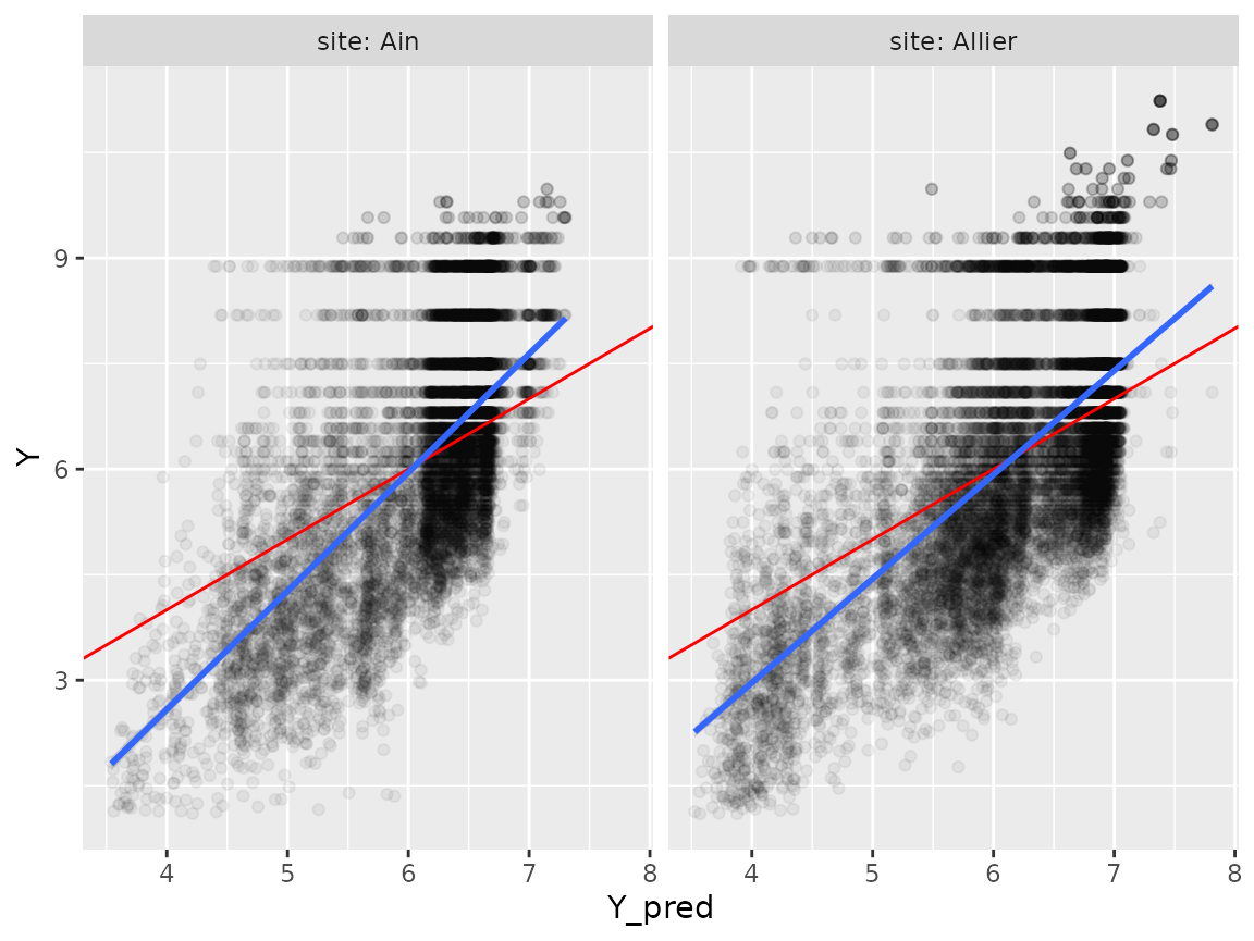

Correction of prediction bias linked to covariate shift

Due to covariate shift, there is a tendency to overestimate low values of Y and underestimate high values of Y (trend in blue, theoretical Y=X line in red).

\[Y=\alpha*Y_{pred}+\beta\]

We will apply a simple linear correction of predictions to account for this in the predict_rf function (arguments)

lm_mod=lm(Y~Y_pred, data=Wdata_pred)
alpha=lm_mod$coefficients[[2]]
beta=lm_mod$coefficients[[1]]
saveRDS(c(alpha,beta),"../data-raw/correction_covariate_shift.RDS")

So we correct \(Y_{pred}\) values accordingly

tib_WpQc=tib_WwtQc %>% 
  mutate(Wdata=purrr::map(.x=Wdata,
                          ~predict_rf(newdata=.x,
                                      obj_rf=myrf,
                                      correction=c(alpha,beta))))

saveRDS(tib_WpQc,"../data-raw/results/tib_WpQc.RDS")

R2=tib_WpQc %>% select(site,Wdata) %>% 
  mutate(R2=purrr::map_df(Wdata,calc_rf_R2)) %>% 
  unnest(R2)
R2

## # A tibble: 2 × 9
## # Groups:   vars, q1.5, station, wpath [2]
##   vars    q1.5 station       wpath            site  Wdata       SCR    SCT    R2
##   <chr>  <dbl> <chr>         <chr>            <chr> <list>    <dbl>  <dbl> <dbl>
## 1 Ain      840 "V294201001 " ../data-raw/Wda… Ain   <tibble> 17575. 31343. 0.439
## 2 Allier   460 "K340081001"  ../data-raw/Wda… Alli… <tibble> 26937. 48109. 0.440

Wdata_pred=tib_WpQc %>% 
  select(Wdata) %>% 
  tidyr::unnest(Wdata, .name_repair="minimal") %>% 
  ungroup() %>% 
  mutate(Ycat=cut(Y,quantile(Y,seq(0,1,by=0.1),include.lowest=TRUE)))

p=ggplot(Wdata_pred,aes(x=Y_pred,y=Y))+
  geom_point(alpha=0.05)+
  geom_abline(intercept=0,slope=1, col="red")+
  facet_grid(cols=vars(site),
             labeller = labeller(.rows = label_both,
                                 .cols = label_both))+
  geom_smooth(method="lm")
plot(p)

15 mars 2022

Global process

For one site

Global process

For several sites

Prepare data

tib_sites: info about wood and discharge data path, and hydrological stations

Wdata : wood occurrence data

Qdata: collect hydrological data & calculate all variables

Qdata completed with calculation of \(T_Q\) and \(S\)

Wdata completed with discharge data

Calculate waiting times to apply random forest model

Prediction

Run random forest on Wdata (both sites)

Predict Wdata based on random forest

Model performance

Plot predicted/observed

Correction of prediction bias linked to covariate shift

`Wdata` : wood occurrence data

`Qdata`: collect hydrological data & calculate all variables

`Qdata` completed with calculation of \(T_Q\) and \(S\)

`Wdata` completed with discharge data