2. woody: calculate flux
15 mars 2022
2._woody_calculate_flux.Rmd
knitr::opts_chunk$set(warning=FALSE,message=FALSE)
library(woody)
library(tidyverse)
library(DiagrammeR)From log-flux estimates \(Y_{pred}\) to flux estimates \(N_{pred}\)
First, let’s see how the predictions of log-flux \(Y_{pred}\) (estimated through the Random Forest) might be used to calculate predictions of flux \(N_{pred}\). It is indeed necessary to take into account the residuals error of the model to do so.
\[Y =log(N)= log(3600/W)\]
where :
- \(N\) is an hourly flux of wood
- \(W\) corresponds to the waiting time(in seconds) between two wood occurrences
- 3600 corresponds to 3600 seconds i.e. one hour
Distribution of \(Y_{pred}\)
Let’s have a look at the distribution of residuals:
tib_WpQc=readRDS("../data-raw/results/tib_WpQc.RDS")
Wdata_pred=tib_WpQc %>%
  select(Wdata) %>%
  tidyr::unnest(Wdata, .name_repair="minimal")

p=ggplot(Wdata_pred,aes(x=Y_pred,y=Y-Y_pred))+
  geom_point(alpha=0.05)+
  facet_grid(cols=vars(site),
             labeller = labeller(.rows = label_both,
                                 .cols = label_both))+
  geom_hline(aes(yintercept=0), col='red')
plot(p)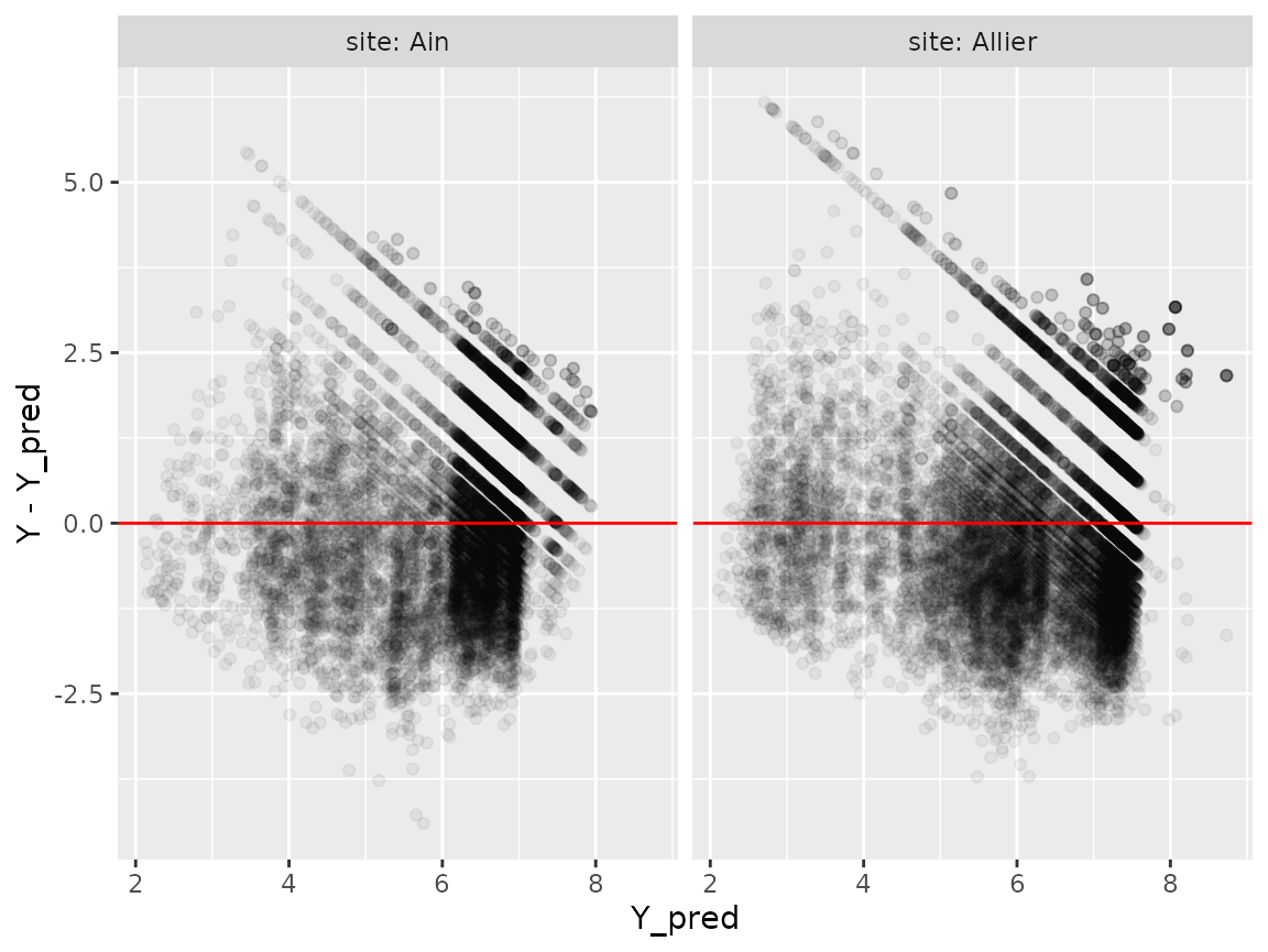
The observed value \(Y\) is distributed around predicted value \(\mu=Y_{pred}\), in an approximately Gaussian distribution:
\[Y=log(3600/W) \sim \mathcal{N}(\mu,\sigma) \] Thus, we have \(log(W)=log(3600)-Y\) hence:
\[log(W) \sim \mathcal{N}(log(3600)-\mu,\sigma) \] The estimate of \(\mu\) is given by
\[\mu=Y_{pred}\] Let us now estimate \(\sigma\).
Estimate of \(\sigma\)
\(\sigma\), as the residual standard deviation, corresponds to a measure of error of the model predicting \(Y\). It actually depends on \(\mu\), as the error tends to be less important when predicted log-flux is important:
data_sigma=Wdata_pred %>%
  ungroup() %>%
  mutate(Ycat=cut(Y_pred,quantile(Y_pred,seq(0,1,by=0.1)))) %>%
  group_by(Ycat) %>%
  summarise(mu=mean(Y_pred),
            sigma=sd(Y_pred-Y))

ggplot(data_sigma, aes(x=mu,y=sigma))+
  geom_point()+
  geom_smooth(method="lm")
lm_sigma=lm(sigma~mu, data=data_sigma)
gamma=lm_sigma$coefficients[[2]]
delta=lm_sigma$coefficients[[1]]
sigma_coeffs=c(gamma,delta)
We will hence consider that
\[\sigma=\gamma\mu+\delta \]
Summarise Qdata hourly and calculate \(N_{pred}\) and \(N_{obs}\)
Interpolate Qdata hourly
Let’s interpolate Qdata at an hourly timescale and use these interpolated, hourly data to calculate \(Y_{pred}\).
Get hourly \(N_{obs}\) and \(N_{obse}\) from Wdata
We want to compare these values \(N_{pred}\) with the observed number of wood pieces during an hour \(N_{obse}\).
The observation of wood pieces is not continuous, so that we have to take into account, for each hour, the proportion of time the observation of wood pieces really occurred \(P_{obs}\). This information is retrievable from Adata (A for “annotation”).
\(N_{obse}=N_{obs}/P_{obs}\)
tib_WnQn=tib_WQn %>%
  mutate(Adata=purrr::map2(.x=apath,.y=site,
                           ~import_Adata(path=.x,site=.y))) %>%
  mutate(Wdata=purrr::map2(.x=Wdata,.y=Adata,
                           ~summarise_Wdata(Wdata=.x,Adata=.y)))
Once imported and cleaned, this how Adata (first lines, for the Ain site) looks like:
| Time | P_obs |
|---|---|
| 2007-11-22 14:00:00 | 0.3166667 |
| 2007-11-22 15:00:00 | 0.1833333 |
| 2007-11-22 16:00:00 | 0.2500000 |
| 2007-11-23 06:00:00 | 0.0544444 |
| 2007-11-23 07:00:00 | 0.2500000 |
| 2007-11-23 08:00:00 | 0.2452778 |
So this is how Wdata now looks like, with a new extrapolated estimate for the observed flux \(N_{obse}\) (first lines, for the Ain site)
| site | event | sitevent | Time | Length | Date | N_obs | P_obs | N_obse |
|---|---|---|---|---|---|---|---|---|
| Ain | event_1 | Ain_event_1 | 2007-11-22 14:00:00 | 1.51 | 2007-11-22 | 3 | 0.3166667 | 9.473684 |
| Ain | event_1 | Ain_event_1 | 2007-11-22 14:00:00 | 1.53 | 2007-11-22 | 3 | 0.3166667 | 9.473684 |
| Ain | event_1 | Ain_event_1 | 2007-11-22 14:00:00 | 4.13 | 2007-11-22 | 3 | 0.3166667 | 9.473684 |
| Ain | event_1 | Ain_event_1 | 2007-11-22 15:00:00 | 5.29 | 2007-11-22 | 1 | 0.1833333 | 5.454546 |
| Ain | event_1 | Ain_event_1 | 2007-11-22 16:00:00 | 1.32 | 2007-11-22 | 1 | 0.2500000 | 4.000000 |
| Ain | event_1 | Ain_event_1 | 2007-11-23 06:00:00 | 3.79 | 2007-11-23 | 22 | 0.0544444 | 404.081633 |
Summary
To make the production of plots easier, we unnest Ndata from tib_WnQnN:
Model performance
R2=tib_WnQnN %>% select(site,Ndata) %>%
  mutate(R2=purrr::map_df(Ndata,calc_rf_R2,type="N")) %>%
  tidyr::unnest(R2)
R2
## # A tibble: 2 × 9
## # Groups: vars, q1.5, station, wpath [2]
## vars q1.5 station wpath site Ndata SCR SCT R2
## <chr> <dbl> <chr> <chr> <chr> <list> <dbl> <dbl> <dbl>
## 1 Ain 840 "V294201001 " ../data-raw/Wda… Ain <tibble> 1.80e8 4.25e8 0.576
## 2 Allier 460 "K340081001" ../data-raw/Wda… Alli… <tibble> 2.81e8 1.06e9 0.736Time plot of \(N_{pred}\) and \(N_{obs}\)
On a log-scale:
Ndataplot=Ndata %>%
  tidyr::pivot_longer(cols=c(N_pred,N_obse), names_to="type") %>%
  filter(!is.na(event))
ggplot(Ndataplot, aes(x=Time,y=value))+
  geom_path(aes(col=type))+
  geom_point(aes(col=type))+
  facet_wrap(site~event, scales="free_x", ncol=1)+
  scale_y_log10()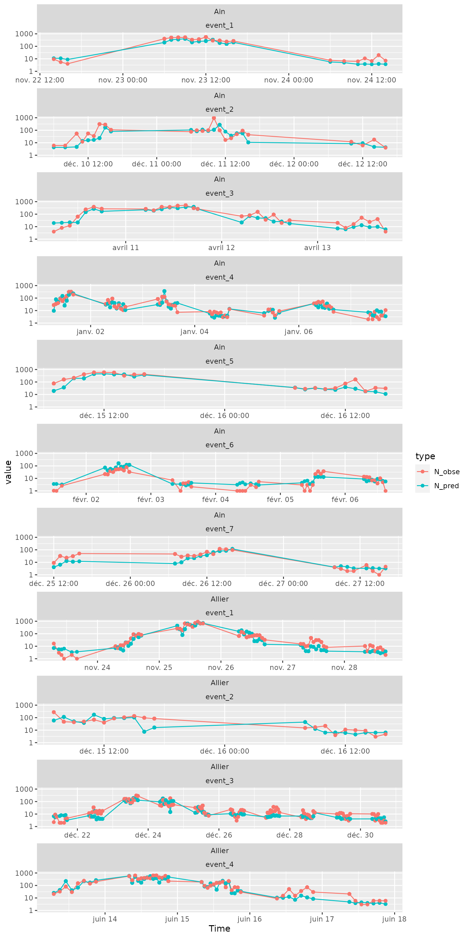
On a natural scale:
Ndataplot=Ndata %>%
  tidyr::pivot_longer(cols=c(N_pred,N_obse), names_to="type") %>%
  filter(!is.na(event))
ggplot(Ndataplot, aes(x=Time,y=value))+
  geom_path(aes(col=type))+
  geom_point(aes(col=type))+
  facet_wrap(site~event, scales="free_x", ncol=1)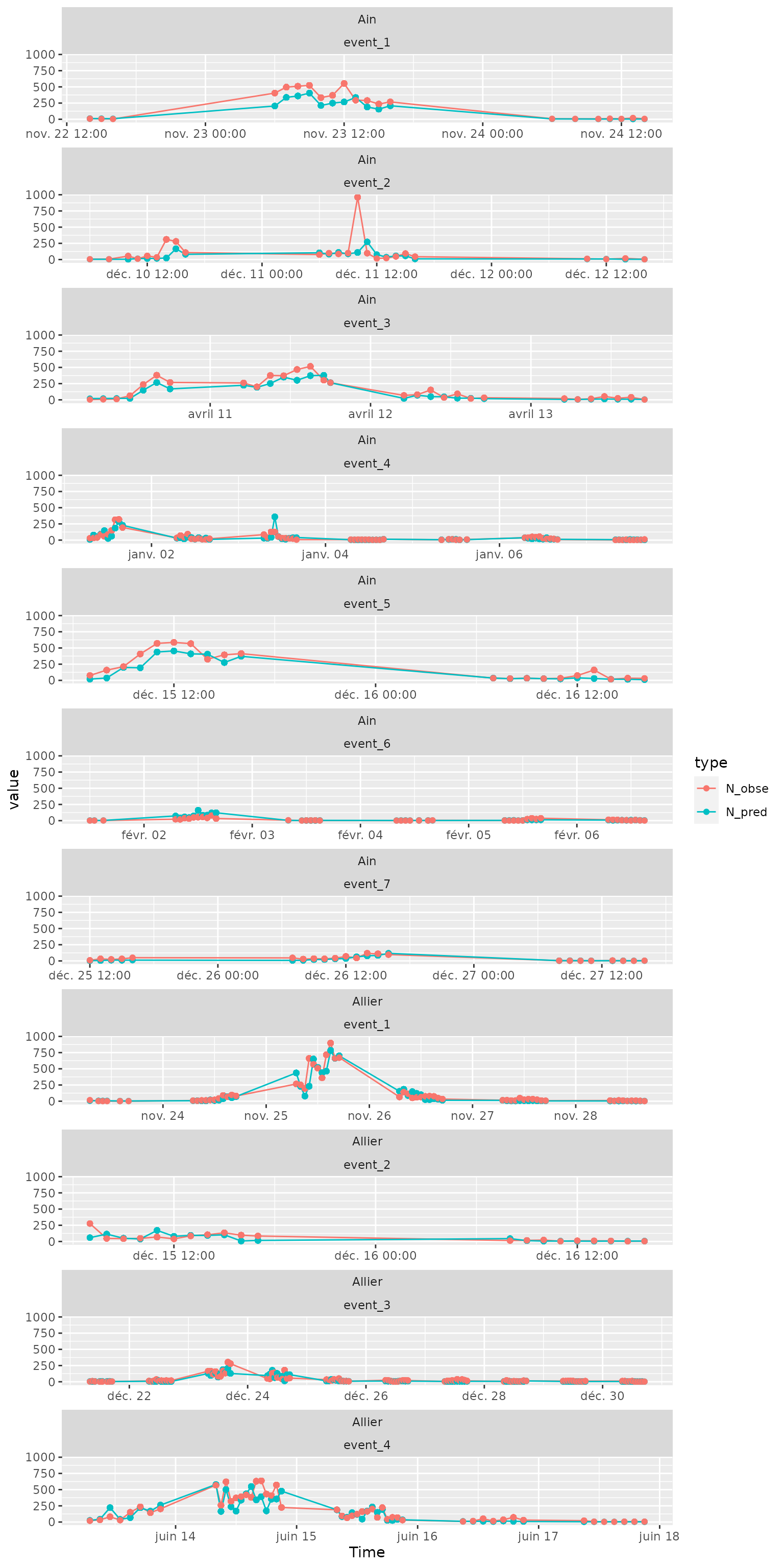
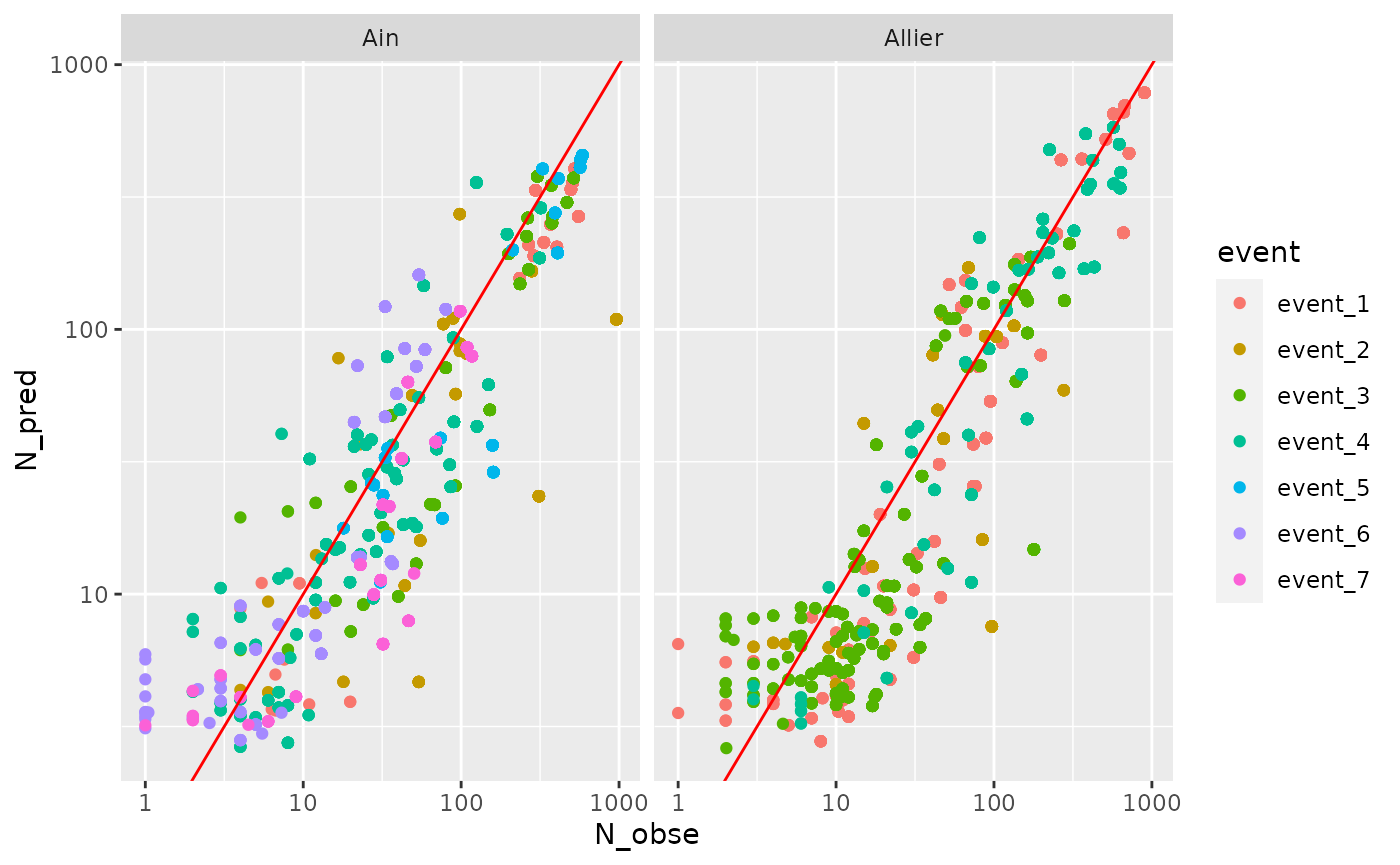
Predicted vs observed (hourly scale)
ggplot(Ndata %>% filter(!is.na(event)), aes(x=N_obse,y=N_pred, col=event))+
  geom_point()+
  geom_abline(vintercept=0,slope=1,col="red")+
  facet_wrap(~site)+
  scale_x_log10()+scale_y_log10()