Variance in the area estimate.
estimation_variance.RmdSources of uncertainty
Now suppose that the series \(s_1\) and \(s_2\) are measured with a certain level of uncertainty, due to
- imprecision in the measure of height \(z\) (\(\sigma_z\)) and/or
- imprecision in the measure of longitudinal coordinate \(l\) (\(\sigma_l\)).
These imprecisions might be different for the two series (change in sampling protocol, improvement in sampling gear between two dates, etc.).
The uncertainty in measures results in a certain amount of uncertainty in the estimate of area between the two curves. This is provided by the function area_uncertainty().
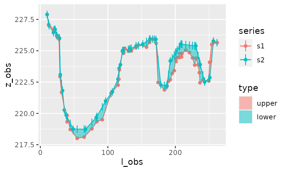
Here, with errors in the measures of height (0.1 and 0.3) higher than in the measures of longitudinal coordinates (0.05 and 0.2), and errors more important for series \(s_2\) (0.3 and 0.2) than for \(s_2\) (0.1 and 0.05).
Estimation of the uncertainty with area_between()
result_area <- area_between(s1,s2,
                            sigma_z=c(0.1,0.3),
                            sigma_l=c(0.05,0.2))
The plot_area() function can provide a visual hint of the uncertainties in \(l\) and \(z\) measures with horizontal and vertical error bars:
plot_area(result_area, show_uncertainty=TRUE)
Here, for instance,
- The estimate of area is -98.07.
- The uncertainty in measures results in an error in the estimate of area of \(\sigma_{area}\)=201.83. Hence we have a 95% confidence interval for the estimate of area of \([A-1.96\cdot\sigma_{area}, A+1.96\cdot\sigma_{area}]\)=[94.15,-290.29].
Check uncertainty through simulation
We can check the calculation of error through a simple simulation with 100 series \(s_{1tmp}\) and \(s_{2tmp}\) varying around \(s_1\) and \(s_2\) respectively, with variations corresponding to estimation errors \(\sigma_z\) and \(\sigma_l\):
set.seed(33)
sigma_z=c(0.1,0.3)
sigma_l=c(0.05,0.2)
f=function(i){
  s1_tmp <- tibble(l=s1$l+rnorm(nrow(s1),0,sigma_l[1]),
                   z=s1$z+rnorm(nrow(s1),0,sigma_z[1]))
  s2_tmp <- tibble(l=s2$l+rnorm(nrow(s2),0,sigma_l[2]),
                   z=s2$z+rnorm(nrow(s2),0,sigma_z[2]))
  return(area_between(s1_tmp,s2_tmp)$area)
}
area_vals=purrr::map_dbl(1:100,f)
sd(area_vals)
#> [1] 14.62939

res=area_between(s1,s2,
                 sigma_z=sigma_z, sigma_l=sigma_l)
res$sigma_area
#> [1] 201.8332