library(riverbed)
library(dplyr)
library(ggplot2)

Load example datasets

Use two transects s1 and s2 already included as example datasets in the package. They correspond to the same place, at two different times.

data(s1)
data(s2)

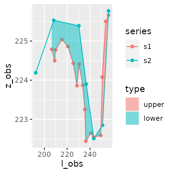
You can compare those two transects and assess the overall change between them through a simple call to area_between().

result_area=area_between(s1,s2)
result_area
#> $data
#> # A tibble: 237 x 13
#>        l    z1 p          z2        a type  l_obs z_obs series  zmin  zmax  lmin
#>    <dbl> <dbl> <chr>   <dbl>    <dbl> <fct> <dbl> <dbl> <chr>  <dbl> <dbl> <dbl>
#>  1  10.1  228. observ…  228.  0       <NA>   10.1  228. s1        NA    NA    NA
#>  2  10.1  228. observ…  228.  8.68e-4 upper  10.1  228. s2        NA    NA    NA
#>  3  10.3  228. inters…  228. NA       upper  NA     NA  <NA>      NA    NA    NA
#>  4  10.3  228. inters…  228. -1.13e-1 lower  NA     NA  <NA>      NA    NA    NA
#>  5  12.3  227. observ…  227.  0       <NA>   12.3  227. s1        NA    NA    NA
#>  6  12.3  227. interp…  227. -2.40e-2 lower  NA     NA  s2        NA    NA    NA
#>  7  12.7  227. inters…  227. NA       lower  NA     NA  <NA>      NA    NA    NA
#>  8  12.7  227. inters…  227.  4.79e-3 upper  NA     NA  <NA>      NA    NA    NA
#>  9  12.9  227. interp…  227.  0       <NA>   NA     NA  s1        NA    NA    NA
#> 10  12.9  227. observ…  227.  1.14e+0 upper  12.9  227. s2        NA    NA    NA
#> # … with 227 more rows, and 1 more variable: lmax <dbl>
#> 
#> $area
#> [1] -98.07248
#> 
#> $area_by_type
#> # A tibble: 2 x 2
#>   type     area
#>   <fct>   <dbl>
#> 1 upper    7.76
#> 2 lower -106.  
#> 
#> $sigma_area
#> [1] 0
plot_area(result_area)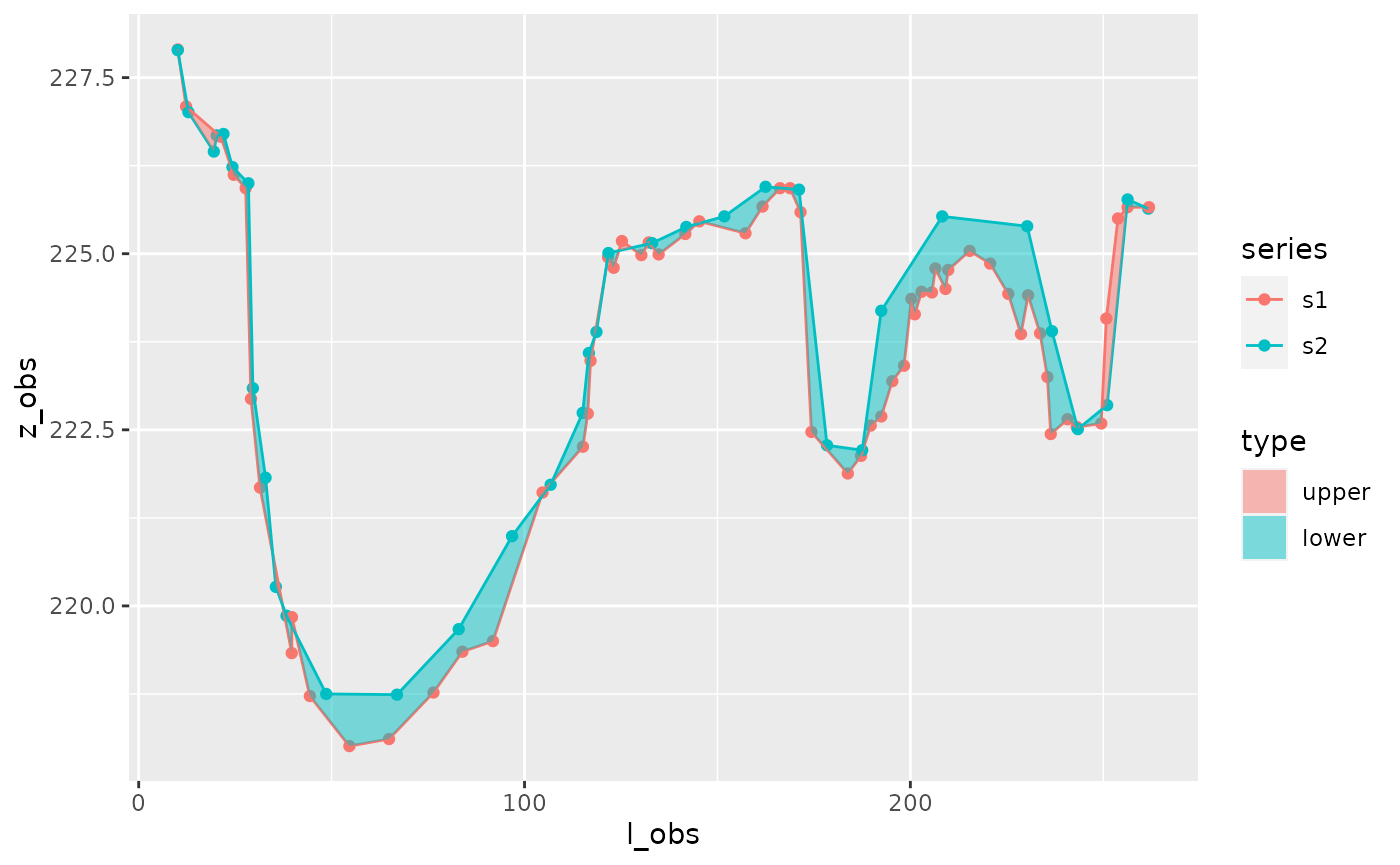

Identify channels with get_channels()

On the other hand, these transects might correspond to a multi-channel riverbed, in which case you might want to assess the changes of each channel individually. It is then necessary to first identify channels.

channels1=get_channels(s1, hmin=1, hmax=5.5)
channels1
#> # A tibble: 3 x 9
#>    id_c   i_a   i_b   l_a   l_b   z_a   z_b z_min z_max
#>   <int> <int> <int> <dbl> <dbl> <dbl> <dbl> <dbl> <dbl>
#> 1     1     5    20  28.2  122.  225.  225.  218.  225.
#> 2     2    32    40 173.   200.  224.  224.  222.  224.
#> 3     3    50    59 231.   251.  224.  224.  222.  224.
plot_channels(channels1,sr=s1)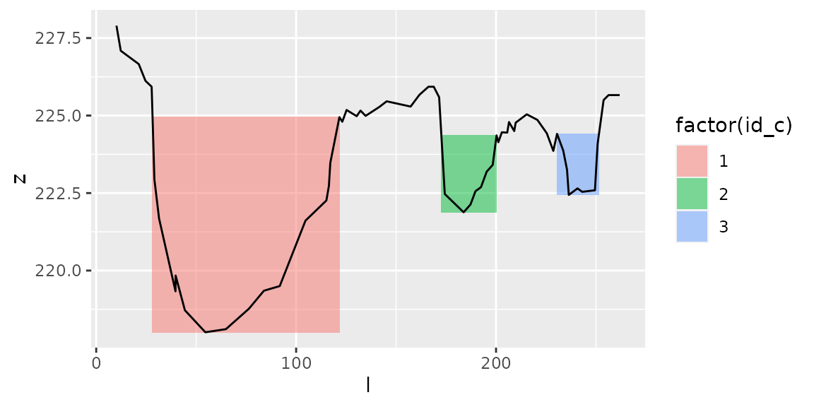

i_a and i_b: indices of observations delimiting the channel,
l_a and l_b: longitudinal coordinates of points delimiting the channel
z_a and z_b: height of points delimiting the channel
z_min and z_max: minimum and maximum height of the channel-delimited profile

The type of channel returned can be either

“bankfull” (the default, as above)
“levee-to-levee” (see example below), which is delimited on both sides by local maxima

Here is what you would get with type=“levee-to-levee”:

channels1=get_channels(s1, hmin=1, hmax=5.5, type="levee-to-levee")
channels1
#> # A tibble: 3 x 9
#>    id_c   i_a   i_b   l_a   l_b   z_a   z_b z_min z_max
#>   <int> <dbl> <dbl> <dbl> <dbl> <dbl> <dbl> <dbl> <dbl>
#> 1     1     1    20  10.1  122.  228.  225.  218.  228.
#> 2     2    31    40 169.   200.  226.  224.  222.  226.
#> 3     3    51    60 231.   256.  224.  226.  222.  226.
plot_channels(channels1,sr=s1)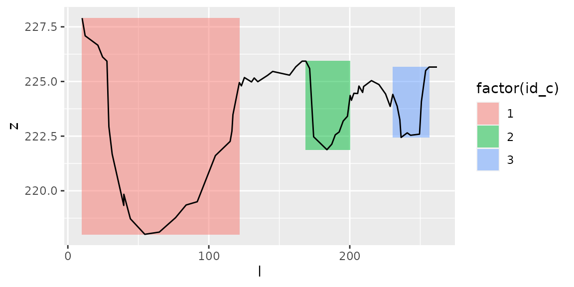

Effect of parameters hmin and hmax

Parameters hmin and hmax

Local minima must be at \(z<z_{min}+h_{max}\) to define a channel’s bottom.

Local maxima must be at \(z>z_{localmin}+h_{min}\) to define a channel’s banks.

Hence \(hmin\) corresponds to the minimum water depth in a channel, and \(hmax\) corresponds to the maximum height of a channel’s bottom.

See the effect of these parameters:

channels1=get_channels(s1, hmin=0.5, hmax=4)
plot_channels(channels1,sr=s1)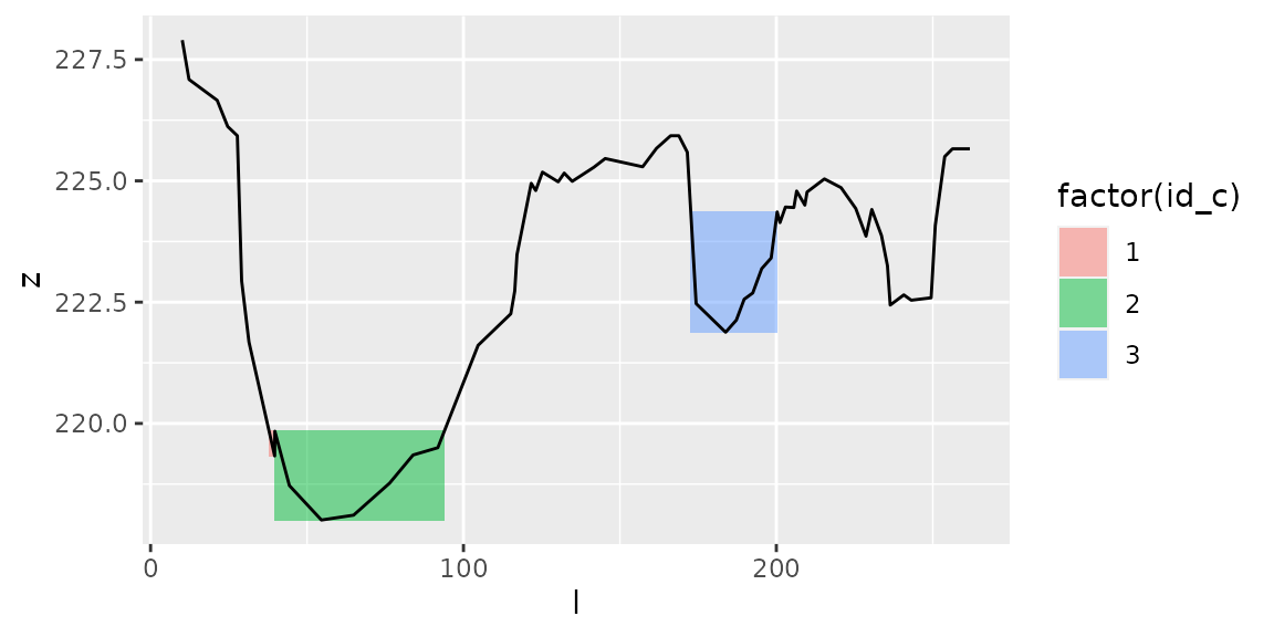

channels1=get_channels(s1, hmin=3, hmax=5)
plot_channels(channels1,sr=s1)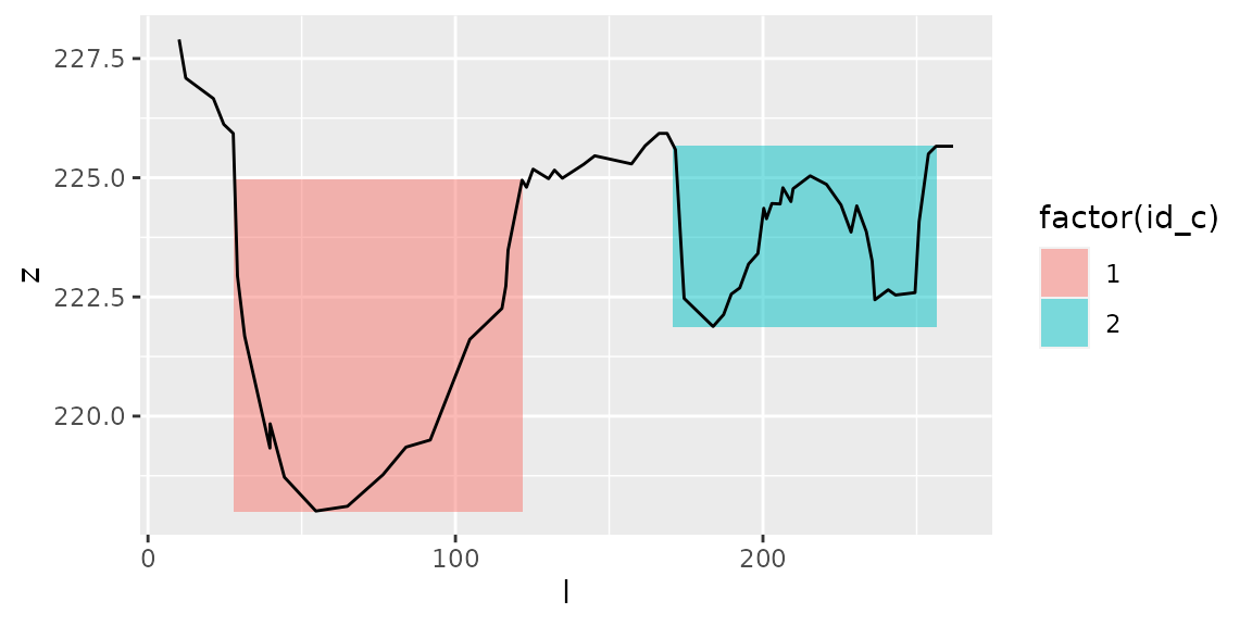

# Regroup channels through dates

Here, with the same values \(h_{min}\) and \(h_{max}\), we get 3 distinct channels at both dates:

channels1=get_channels(s1,hmin=1,hmax=5.5)
plot_channels(channels1,sr=s1)

channels2=get_channels(s2,hmin=1,hmax=5.5)
plot_channels(channels2,sr=s2)

… But these correspond to different \(l\) coordinates.

So, we have to somehow “regroup” these coordinates to be able to compare the transects with channel-wise area calculations.

Example of channel-wise area calculation through two dates

get_channels()

Let’s apply the get_channels() function to all transects (the column identifying those being called “id_transect”).

transects=bind_rows(bind_cols(id_transect="s1",s1),
                    bind_cols(id_transect="s2",s2))%>% 
  group_by(id_transect) %>% 
  tidyr::nest()

The table transects gathers the data of both transects s1 and s2. Let’s apply get_channels() iteratively to each transect:

channels =transects %>%  
  mutate(data=purrr::map(data,get_channels, hmin=1, hmax=4.5)) %>% 
  tidyr::unnest(cols=data) 
channels
#> # A tibble: 6 x 10
#> # Groups:   id_transect [2]
#>   id_transect  id_c   i_a   i_b   l_a   l_b   z_a   z_b z_min z_max
#>   <chr>       <int> <int> <int> <dbl> <dbl> <dbl> <dbl> <dbl> <dbl>
#> 1 s1              1     5    20  28.2  122.  225.  225.  218.  225.
#> 2 s1              2    32    40 173.   200.  224.  224.  222.  224.
#> 3 s1              3    50    59 231.   251.  224.  224.  222.  224.
#> 4 s2              1     7    24  28.5  162.  226.  226.  219.  226.
#> 5 s2              2    25    30 172.   208.  226.  226.  222.  226.
#> 6 s2              3    28    34 208.   256.  226.  226.  223.  226.

regroup_channels()

Both transects correspond to 3 channels with identifier id_c (1,2,3).

We regroup these channels with function regroup_channels(), which returns for each channel longitudinal limits l_a and l_b. These limits include the total width of both channels.

regrouped_channels=regroup_channels(channels,by_id=id_c)
regrouped_channels
#> # A tibble: 3 x 3
#>    id_c   l_a   l_b
#>   <int> <dbl> <dbl>
#> 1     1  28.2  162.
#> 2     2 172.   208.
#> 3     3 208.   256.
plot_channels(channels1, s1)+
  geom_vline(data=regrouped_channels, aes(xintercept=l_a), col="grey")+
  geom_vline(data=regrouped_channels, aes(xintercept=l_b), col="grey")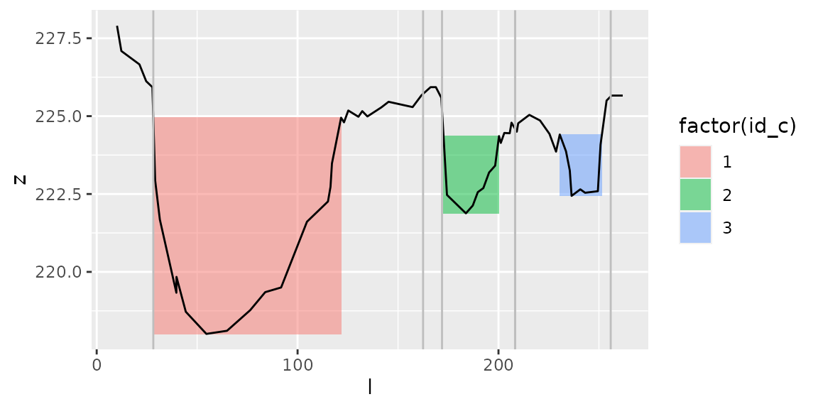

plot_channels(channels2, s2)+
  geom_vline(data=regrouped_channels, aes(xintercept=l_a), col="grey")+
  geom_vline(data=regrouped_channels, aes(xintercept=l_b), col="grey")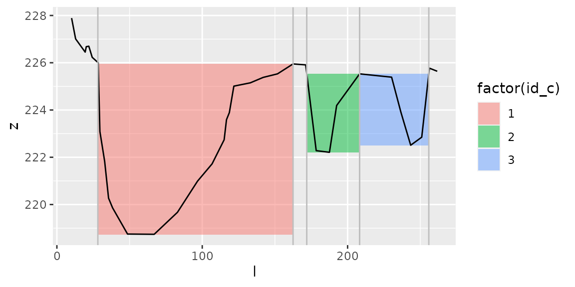

## area_between()

areas_result=transects %>%
  mutate(subdata=purrr::map(data,cut_series,
                            channels=regrouped_channels)) %>% 
  tidyr::unnest(cols=subdata) %>% 
  tidyr::pivot_wider(id_cols=id_c, names_from=id_transect,values_from=sr) %>%
  mutate(area_complete=purrr::map2(s1,s2,area_between))
areas_result
#> # A tibble: 3 x 4
#>    id_c s1                s2                area_complete   
#>   <int> <list>            <list>            <list>          
#> 1     1 <tibble [26 × 2]> <tibble [19 × 2]> <named list [4]>
#> 2     2 <tibble [14 × 2]> <tibble [6 × 2]>  <named list [4]>
#> 3     3 <tibble [17 × 2]> <tibble [7 × 2]>  <named list [4]>

format result

areas_formatted_result= areas_result%>%
  mutate(area=purrr::map_dbl(area_complete,~.x$area)) %>% 
  mutate(area_lower=purrr::map_dbl(area_complete,
                                   ~.x$area_by_type %>%
                                     filter(type=="lower") %>% pull(area))) %>% 
  mutate(area_upper=purrr::map_dbl(area_complete,
                                   ~.x$area_by_type %>% 
                                     filter(type=="upper") %>% pull(area))) %>% 
  mutate(plot=purrr::map(area_complete,plot_area)) %>% 
  select(id_c,area,area_lower,area_upper,plot)
areas_formatted_result
#> # A tibble: 3 x 5
#>    id_c  area area_lower area_upper plot  
#>   <int> <dbl>      <dbl>      <dbl> <list>
#> 1     1 -47.8      -48.6      0.800 <gg>  
#> 2     2 -27.9      -27.9      0     <gg>  
#> 3     3 -23.9      -29.6      5.66  <gg>

areas_formatted_result$plot
#> [[1]]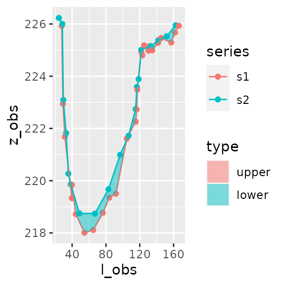

#> 
#> [[2]]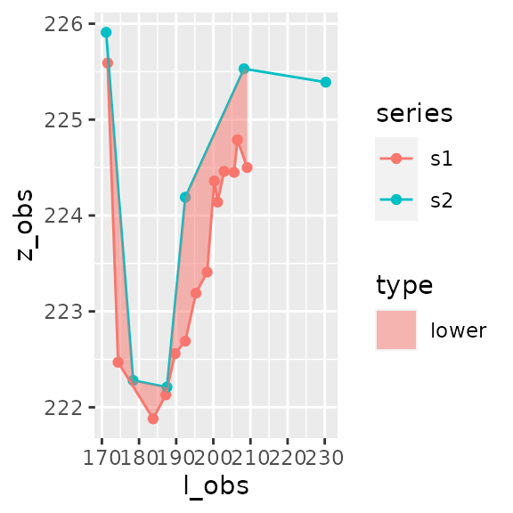

#> 
#> [[3]]