4. Normalization

Normalizing the data

We continue the Seurat tutorial on the analysis of Peripheral Blood Mononuclear Cells (PBMC) at the Normalizing the data step.

What is the difference between the two following commands ?

pbmc <- NormalizeData(pbmc, normalization.method = "LogNormalize", scale.factor = 10000)

pbmc <- SCTransform(pbmc, vars.to.regress = "percent.mt", verbose = FALSE)

Which one would you choose for your analysis ?

The following plot represents the relationship between the genes mean and variance across cells.

library(tidyverse)
library(Seurat)
library(SeuratData)
InstallData("pbmc3k")
data("pbmc3k")
pbmc3k <- UpdateSeuratObject(pbmc3k)

tibble(
  cell_mean = rowMeans(pbmc3k@assays$RNA@counts),
  cell_var = apply(pbmc3k@assays$RNA@counts, 1, var)
) %>% 
  ggplot(aes(x = log(cell_mean), y = log(cell_var))) +
  geom_point(alpha=0.3) +
  geom_abline(intercept = 0,
              slope = 1,
              color = 'red') +
  theme_bw()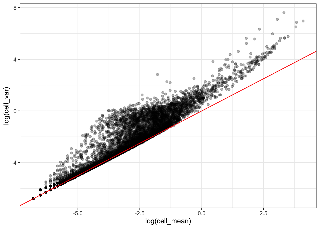

What can you tell about this relationship ?

To which model corresponds the red line ?

In their paper Choudhary & Satija 2022 describe the SCTransform method in the Modeling scRNA-seq datasets with sctransform subsection of the Methods section.

What additional factors would you add in addition to \(n_c\) in the generalized linear model (GLM) used by SCTransform ?

Identification of highly variable features (feature selection)

Look for a description of the "vst" method

pbmc <- FindVariableFeatures(pbmc, selection.method = "vst", nfeatures = 2000)

Why do we need to select the \(2000\) most variable genes ?

How could this be a problem ?

In their paper Breda et al. 2021 show by extensive simulation that we cannot get a reliable variance estimator, in scRNAseq data, for genes \(j\) with: \[\frac{1}{n}\sum_{i=1}^{n}x_i \leq 1\]

Knowing that how could you select which genes to analyze ?

How could this be a problem ?

In the next section where you will learn how to represent scRNASeq data.