Systematic differences in sequencing coverage between libraries are often observed in single-cell RNA sequencing data. They typically arise from technical differences in cDNA capture or PCR amplification efficiency across cells, attributable to the difficulty of achieving consistent library preparation with minimal starting material. Normalization aims to remove these differences such that they do not interfere with comparisons of the expression profiles between cells. This ensures that any observed heterogeneity or differential expression within the cell population is driven by biology and not technical biases.
We will now calculate some properties and visually inspect the data. Our main interest is in the general trends not in individual outliers. Neither genes nor cells that stand out are important at this step, but we focus on the global trends.
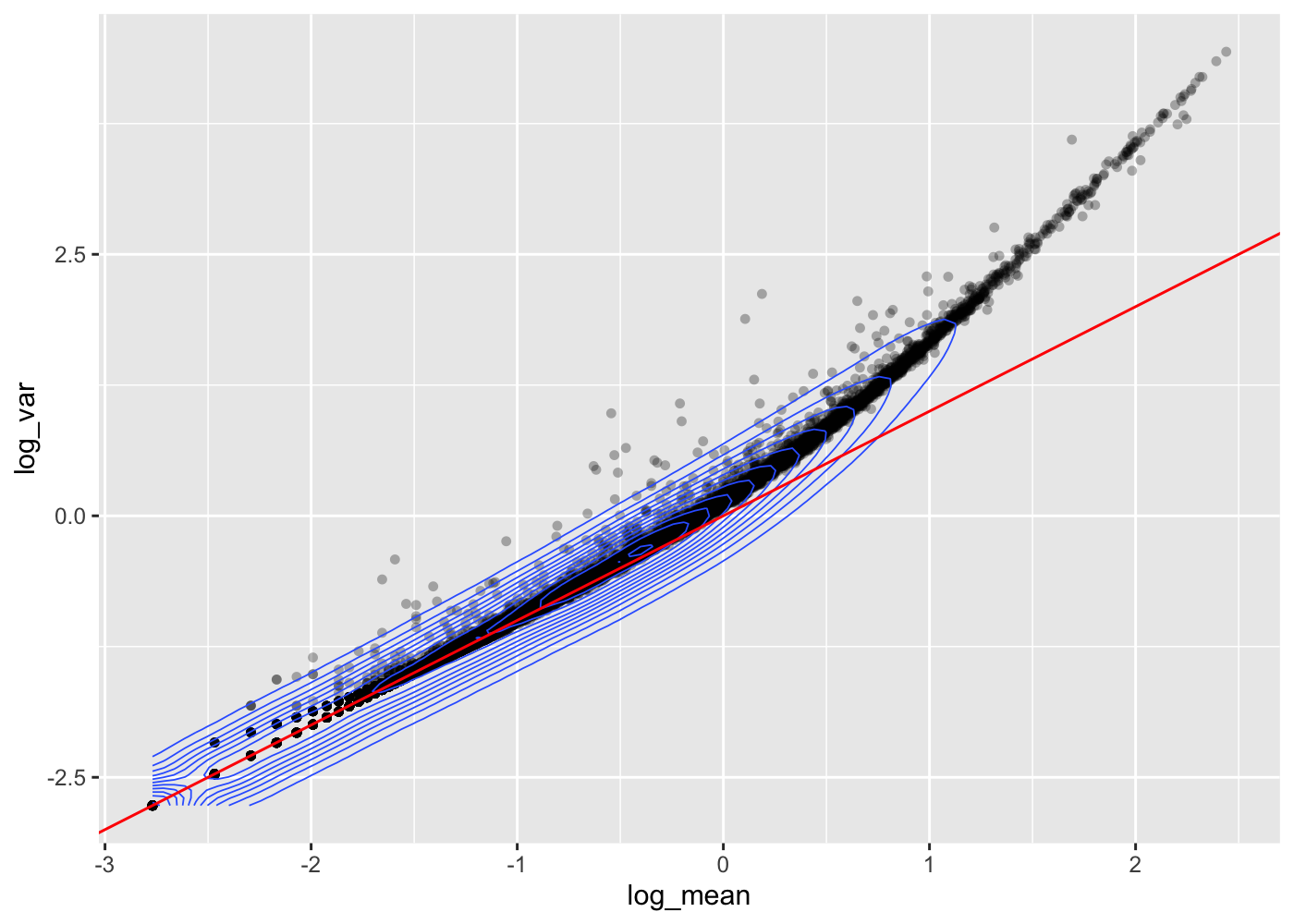
Derive gene and cell attributes from the UMI matrix to plot the mean-variance relationship (on the expressed gene and non-empty droplets in log scale).
From this mean-variance relationship, we can see that up to a given mean UMI count the variance follows the line through the origin with slop one, i.e. variance and mean are roughly equal as expected under a Poisson model. However, genes with a higher average UMI count show overdispersion compared to Poisson.
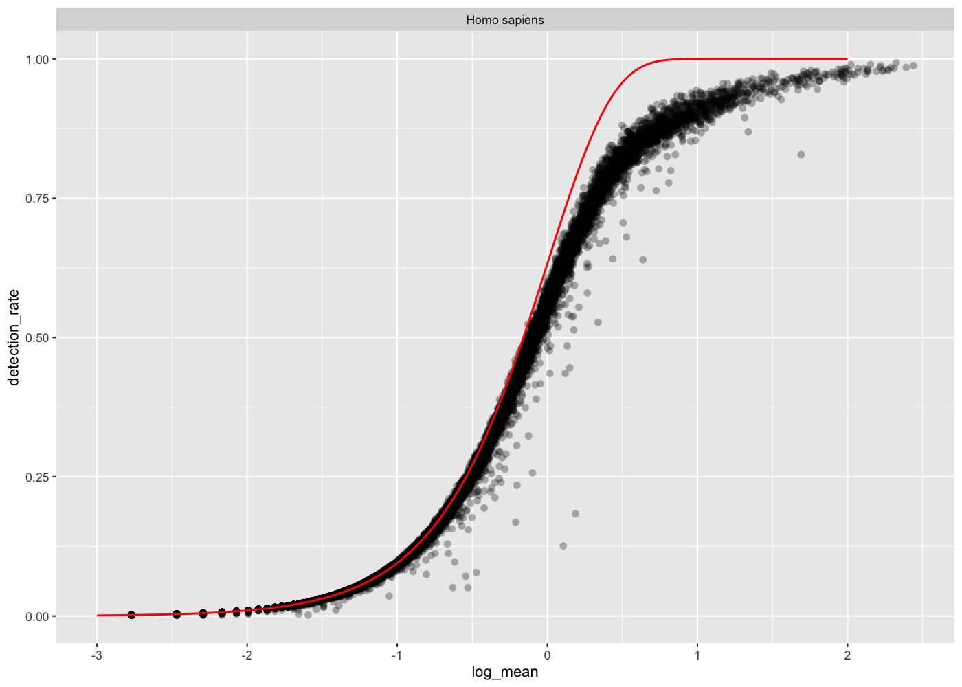
The sampling process of each gene depending on its mean expression can be modeled with a Poisson. You can plot this theoretical detection rate and compare it to the empirical detection rate of each gene.
# add the expected detection rate under Poisson modelx =seq(from =-3, to =2, length.out =1000)poisson_model <-tibble(log_mean = x,detection_rate =1-dpois(0, lambda =10^ x))rowData(sce_hg) %>%as_tibble() %>% dplyr::filter(is_genomic) %>%ggplot(aes(x = log_mean, y = detection_rate)) +geom_point(alpha =0.3, shape =16) +geom_line(data = poisson_model, color ='red') +theme_gray(base_size =8) +facet_wrap(~species)
From the mean-detection-rate relationship, we see a lower than expected detection rate in the medium expression range. However, for the highly expressed genes, the rate is at or very close to 1.0 suggesting that there is no zero-inflation in the counts for those genes and that zero-inflation is a result of overdispersion, rather than an independent systematic bias.
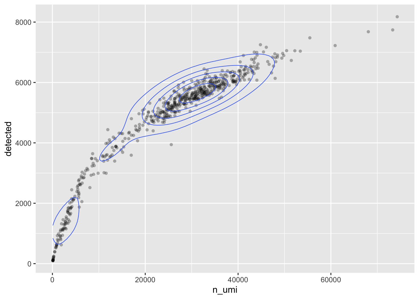
The more UMI counts a cell has, the more genes are detected. In this data set, this seems to be an almost linear relationship (at least within the UMI range of most of the cells).
The scTransform transform algorithms, Hafemeister et al. 2019 propose to model the expression of each gene as a negative binomial random variable with a mean that depends on other variables. Here the other variables can be used to model the differences in sequencing depth between cells and are used as independent variables in a regression model. In order to avoid overfitting, we will first fit model parameters per gene, and then use the relationship between gene mean and parameter values to fit parameters, thereby combining information across genes. Given the fitted model parameters, we transform each observed UMI count into a Pearson residual which can be interpreted as the number of standard deviations an observed count was away from the expected mean. If the model accurately describes the mean-variance relationship and the dependency of mean and latent factors, then the result should have mean zero and a stable variance across the range of expression.
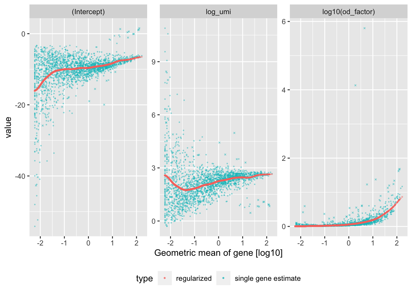
The vst() function estimates model parameters and performs the variance stabilizing transformation. Here we use the log10 of the total UMI counts of a cell as variable for sequencing depth for each cell. After data transformation we plot the model parameters as a function of gene mean (geometric mean). The correct() function computes the corrected count matrix.
Internally vst performs Poisson regression per gene with \(\log(\mu) = \beta_0 + \beta_1 x\), where \(x\) is log_umi, the base 10 logarithm of the total number of UMI counts in each cell, and μ are the expected number of UMI counts of the given gene. The previous plot shows \(\beta_0\)(Intercept), the \(\beta_1\) coefficient log_umi, and the maximum likelihood estimate of the overdispersion parameter theta under the negative binomial model. Under the negative binomial model, the variance of a gene depends on the expected UMI counts and theta: \(\mu + \frac{\mu^2}{\theta}\). In a second step, the regularized model parameters are used to turn observed UMI counts into Pearson residuals.
After exploring the problem of empty droplets and doublets. We now turn toward another scRNASeq data set to exploit another aspect of scRNASeq data.